Apache Kudu Schema Design

This document applies to Apache Kudu version 1.17.1. Please consult the documentation of the appropriate release that’s applicable to the version of the Kudu cluster.

Overview

Kudu tables have a structured data model similar to tables in a traditional RDBMS. Schema design is critical for achieving the best performance and operational stability from Kudu. Every workload is unique, and there is no single schema design that is best for every table. This document outlines effective schema design philosophies for Kudu, paying particular attention to where they differ from approaches used for traditional RDBMS schemas.

At a high level, there are three concerns when creating Kudu tables: column design, primary key design, and partitioning design. Of these, only partitioning will be a new concept for those familiar with traditional non-distributed relational databases. The final sections discuss altering the schema of an existing table, and known limitations with regard to schema design.

The Perfect Schema

The perfect schema would accomplish the following:

Data would be distributed in such a way that reads and writes are spread evenly across tablet servers. This is impacted by partitioning.
Tablets would grow at an even, predictable rate and load across tablets would remain steady over time. This is most impacted by partitioning.
Scans would read the minimum amount of data necessary to fulfill a query. This is impacted mostly by primary key design, but partitioning also plays a role via partition pruning.

The perfect schema depends on the characteristics of your data, what you need to do with it, and the topology of your cluster. Schema design is the single most important thing within your control to maximize the performance of your Kudu cluster.

Column Design

A Kudu Table consists of one or more columns, each with a defined type. Columns that are not part of the primary key may be nullable. Supported column types include:

boolean
8-bit signed integer
16-bit signed integer
32-bit signed integer
64-bit signed integer
date (32-bit days since the Unix epoch)
unixtime_micros (64-bit microseconds since the Unix epoch)
single-precision (32-bit) IEEE-754 floating-point number
double-precision (64-bit) IEEE-754 floating-point number
decimal (see Decimal Type for details)
varchar (see Varchar Type for details)
UTF-8 encoded string (up to 64KB uncompressed)
binary (up to 64KB uncompressed)

Kudu takes advantage of strongly-typed columns and a columnar on-disk storage format to provide efficient encoding and serialization. To make the most of these features, columns should be specified as the appropriate type, rather than simulating a 'schemaless' table using string or binary columns for data which may otherwise be structured. In addition to encoding, Kudu allows compression to be specified on a per-column basis.

No Version or Timestamp Column

Kudu does not provide a version or timestamp column to track changes to a row. If version or timestamp information is needed, the schema should include an explicit version or timestamp column.

Decimal Type

The decimal type is a numeric data type with fixed scale and precision suitable for financial and other arithmetic calculations where the imprecise representation and rounding behavior of float and double make those types impractical. The decimal type is also useful for integers larger than int64 and cases with fractional values in a primary key.

The decimal type is a parameterized type that takes precision and scale type attributes.

Precision represents the total number of digits that can be represented by the column, regardless of the location of the decimal point. This value must be between 1 and 38 and has no default. For example, a precision of 4 is required to represent integer values up to 9999, or to represent values up to 99.99 with two fractional digits. You can also represent corresponding negative values, without any change in the precision. For example, the range -9999 to 9999 still only requires a precision of 4.

Scale represents the number of fractional digits. This value must be between 0 and the precision. A scale of 0 produces integral values, with no fractional part. If precision and scale are equal, all of the digits come after the decimal point. For example, a decimal with precision and scale equal to 3 can represent values between -0.999 and 0.999.

Performance considerations:

Kudu stores each value in as few bytes as possible depending on the precision specified for the decimal column. For that reason it is not advised to just use the highest precision possible for convenience. Doing so could negatively impact performance, memory and storage.

Before encoding and compression:

Decimal values with precision of 9 or less are stored in 4 bytes.
Decimal values with precision of 10 through 18 are stored in 8 bytes.
Decimal values with precision greater than 18 are stored in 16 bytes.

The precision and scale of decimal columns cannot be changed by altering the table.

Varchar Type

The varchar type is a UTF-8 encoded string (up to 64KB uncompressed) with a fixed maximum character length. This type is especially useful when migrating from or integrating with legacy systems that support the varchar type. If a maximum character length is not required the string type should be used instead.

The varchar type is a parameterized type that takes a length attribute.

Length represents the maximum number of UTF-8 characters allowed. Values with characters greater than the limit will be truncated. This value must be between 1 and 65535 and has no default. Note that some other systems may represent the length limit in bytes instead of characters. That means that Kudu may be able to represent longer values in the case of multi-byte UTF-8 characters.

Column Encoding

Each column in a Kudu table can be created with an encoding, based on the type of the column.

Table 1. Encoding Types
Column Type	Encoding	Default
int8, int16, int32, int64	plain, bitshuffle, run length	bitshuffle
date, unixtime_micros	plain, bitshuffle, run length	bitshuffle
float, double, decimal	plain, bitshuffle	bitshuffle
bool	plain, run length	run length
string, varchar, binary	plain, prefix, dictionary	dictionary

Plain Encoding: Data is stored in its natural format. For example, int32 values are stored as fixed-size 32-bit little-endian integers.

Bitshuffle Encoding: A block of values is rearranged to store the most significant bit of every value, followed by the second most significant bit of every value, and so on. Finally, the result is LZ4 compressed. Bitshuffle encoding is a good choice for columns that have many repeated values, or values that change by small amounts when sorted by primary key. The bitshuffle project has a good overview of performance and use cases.

Run Length Encoding: Runs (consecutive repeated values) are compressed in a column by storing only the value and the count. Run length encoding is effective for columns with many consecutive repeated values when sorted by primary key.

Dictionary Encoding: A dictionary of unique values is built, and each column value is encoded as its corresponding index in the dictionary. Dictionary encoding is effective for columns with low cardinality. If the column values of a given row set are unable to be compressed because the number of unique values is too high, Kudu will transparently fall back to plain encoding for that row set. This is evaluated during flush.

Prefix Encoding: Common prefixes are compressed in consecutive column values. Prefix encoding can be effective for values that share common prefixes, or the first column of the primary key, since rows are sorted by primary key within tablets.

Column Compression

Kudu allows per-column compression using the LZ4, Snappy, or zlib compression codecs. By default, columns that are Bitshuffle-encoded are inherently compressed with LZ4 compression. Otherwise, columns are stored uncompressed. Consider using compression if reducing storage space is more important than raw scan performance.

Every data set will compress differently, but in general LZ4 is the most performant codec, while zlib will compress to the smallest data sizes. Bitshuffle-encoded columns are automatically compressed using LZ4, so it is not recommended to apply additional compression on top of this encoding.

Primary Key Design

Every Kudu table must declare a primary key comprised of one or more columns. Like an RDBMS primary key, the Kudu primary key enforces a uniqueness constraint. Attempting to insert a row with the same primary key values as an existing row will result in a duplicate key error.

Primary key columns must be non-nullable, and may not be a boolean, float or double type.

Once set during table creation, the set of columns in the primary key may not be altered.

Unlike an RDBMS, Kudu does not provide an explicit auto-incrementing column feature, so the application must always provide the full primary key during insert.

Columns which do not satisfy the uniqueness constraint can still be used as primary keys, by specifying them as non-unique primary keys.

Row delete and update operations must also specify the full primary key of the row to be changed. Kudu does not natively support range deletes or updates.

The primary key values of a column may not be updated after the row is inserted. However, the row may be deleted and re-inserted with the updated value.

Primary Key Index

As with many traditional relational databases, Kudu’s primary key is in a clustered index. All rows within a tablet are sorted by its primary key.

When scanning Kudu rows, use equality or range predicates on primary key columns to efficiently find the rows.

Primary key indexing optimizations apply to scans on individual tablets. See the Partition Pruning section for details on how scans can use predicates to skip entire tablets.

Non-unique Primary Key Index

While specifying columns as non-unique primary key, Kudu internally creates an auto-incrementing column. The specified columns and the auto-incrementing column form the effective primary key.

The auto-incrementing counter which is used to assign value for auto-incrementing column is managed by Kudu, the counter values are monotonically increasing per tablet.

Non-unique primary key columns must be non-nullable, and may not be a boolean, float or double type.

Once set during table creation, the set of columns in the non-unique primary key and the auto-incrementing column can not be altered.

For inserts, one has to provide values for the non-unique primary key columns without specifying the values for auto-incrementing column. The auto-incrementing column is populated on the server side automatically.

For updates/deletes the full set of key columns is necessary. One has to perform a scan before update/delete operation to get the auto-incrementing value.

Upsert operation is not supported on tables with non-unique primary key.

The non-unique primary key values of a column may not be updated after the row is inserted. However, the row may be deleted and re-inserted with the updated value, moreover a new auto-incrementing counter value is assigned during insertion for auto-incrementing column.

Restoring tables with non-unique primary keys is not supported currently.

For more details on how to use non-unique primary key, please check the examples folder.

Considerations for Backfill Inserts

This section discuss a primary key design consideration for timeseries use cases where the primary key is a timestamp, or the first column of the primary key is a timestamp.

Each time a row is inserted into a Kudu table, Kudu looks up the primary key in the primary key index storage to check whether that primary key is already present in the table. If the primary key exists in the table, a "duplicate key" error is returned. In the typical case where data is being inserted at the current time as it arrives from the data source, only a small range of primary keys are "hot". So, each of these "check for presence" operations is very fast. It hits the cached primary key storage in memory and doesn’t require going to disk.

In the case when you load historical data, which is called "backfilling", from an offline data source, each row that is inserted is likely to hit a cold area of the primary key index which is not resident in memory and will cause one or more HDD disk seeks. For example, in a normal ingestion case where Kudu sustains a few million inserts per second, the "backfill" use case might sustain only a few thousand inserts per second.

To alleviate the performance issue during backfilling, consider the following options:

Make the primary keys more compressible.

For example, with the first column of a primary key being a random ID of 32-bytes, caching one billion primary keys would require at least 32 GB of RAM to stay in cache. If caching backfill primary keys from several days ago, you need to have several times 32 GB of memory. By changing the primary key to be more compressible, you increase the likelihood that the primary keys can fit in cache and thus reducing the amount of random disk I/Os.
Use SSDs for storage as random seeks are orders of magnitude faster than spinning disks.
Change the primary key structure such that the backfill writes hit a continuous range of primary keys.

Partitioning

In order to provide scalability, Kudu tables are partitioned into units called tablets, and distributed across many tablet servers. A row always belongs to a single tablet. The method of assigning rows to tablets is determined by the partitioning of the table, which is set during table creation.

Choosing a partitioning strategy requires understanding the data model and the expected workload of a table. For write-heavy workloads, it is important to design the partitioning such that writes are spread across tablets in order to avoid overloading a single tablet. For workloads involving many short scans, where the overhead of contacting remote servers dominates, performance can be improved if all of the data for the scan is located in the same tablet. Understanding these fundamental trade-offs is central to designing an effective partition schema.

No Default Partitioning

Kudu does not provide a default partitioning strategy when creating tables. It is recommended that new tables which are expected to have heavy read and write workloads have at least as many tablets as tablet servers.

Kudu provides two types of partitioning: range partitioning and hash partitioning. Tables may also have multilevel partitioning, which combines range and hash partitioning, or multiple instances of hash partitioning.

Range Partitioning

Range partitioning distributes rows using a totally-ordered range partition key. Each partition is assigned a contiguous segment of the range partition keyspace. The key must be comprised of a subset of the primary key columns. If the range partition columns match the primary key columns, then the range partition key of a row will equal its primary key. In range partitioned tables without hash partitioning, each range partition will correspond to exactly one tablet.

The initial set of range partitions is specified during table creation as a set of partition bounds and split rows. For each bound, a range partition will be created in the table. Each split will divide a range partition in two. If no partition bounds are specified, then the table will default to a single partition covering the entire key space (unbounded below and above). Range partitions must always be non-overlapping, and split rows must fall within a range partition.

see the Range Partitioning Example for further discussion of range partitioning.

Range Partition Management

Kudu allows range partitions to be dynamically added and removed from a table at runtime, without affecting the availability of other partitions. Removing a partition will delete the tablets belonging to the partition, as well as the data contained in them. Subsequent inserts into the dropped partition will fail. New partitions can be added, but they must not overlap with any existing range partitions. Kudu allows dropping and adding any number of range partitions in a single transactional alter table operation.

Dynamically adding and dropping range partitions is particularly useful for time series use cases. As time goes on, range partitions can be added to cover upcoming time ranges. For example, a table storing an event log could add a month-wide partition just before the start of each month in order to hold the upcoming events. Old range partitions can be dropped in order to efficiently remove historical data, as necessary.

Hash Partitioning

Hash partitioning distributes rows by hash value into one of many buckets. In single-level hash partitioned tables, each bucket will correspond to exactly one tablet. The number of buckets is set during table creation. Typically the primary key columns are used as the columns to hash, but as with range partitioning, any subset of the primary key columns can be used.

Hash partitioning is an effective strategy when ordered access to the table is not needed. Hash partitioning is effective for spreading writes randomly among tablets, which helps mitigate hot-spotting and uneven tablet sizes.

see the Hash Partitioning Example for further discussion of hash partitioning.

Multilevel Partitioning

Kudu allows a table to combine multiple levels of partitioning on a single table. Zero or more hash partition levels can be combined with an optional range partition level. The only additional constraint on multilevel partitioning beyond the constraints of the individual partition types, is that multiple levels of hash partitions must not hash the same columns.

When used correctly, multilevel partitioning can retain the benefits of the individual partitioning types, while reducing the downsides of each. The total number of tablets in a multilevel partitioned table is the product of the number of partitions in each level.

see the Hash and Range Partitioning Example and the Hash and Hash Partitioning Example for further discussion of multilevel partitioning.

Partition Pruning

Kudu scans will automatically skip scanning entire partitions when it can be determined that the partition can be entirely filtered by the scan predicates. To prune hash partitions, the scan must include equality predicates on every hashed column. To prune range partitions, the scan must include equality or range predicates on the range partitioned columns. Scans on multilevel partitioned tables can take advantage of partition pruning on any of the levels independently.

Partitioning Examples

To illustrate the factors and trade-offs associated with designing a partitioning strategy for a table, we will walk through some different partitioning scenarios. Consider the following table schema for storing machine metrics data (using SQL syntax and date-formatted timestamps for clarity):

CREATE TABLE metrics (
    host STRING NOT NULL,
    metric STRING NOT NULL,
    time INT64 NOT NULL,
    value DOUBLE NOT NULL,
    PRIMARY KEY (host, metric, time)
);

Range Partitioning Example

A natural way to partition the metrics table is to range partition on the time column. Let’s assume that we want to have a partition per year, and the table will hold data for 2014, 2015, and 2016. There are at least two ways that the table could be partitioned: with unbounded range partitions, or with bounded range partitions.

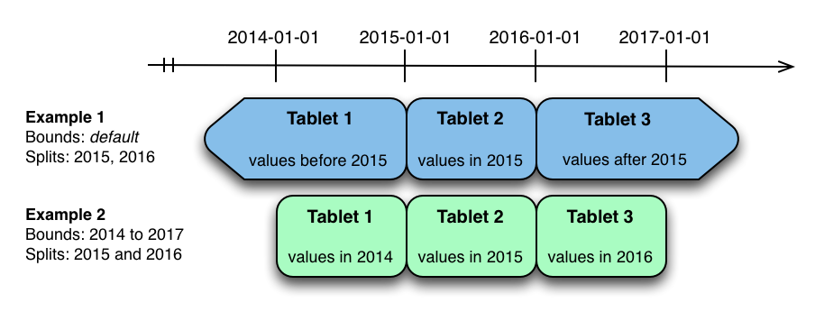
The image above shows the two ways the metrics table can be range partitioned on the time column. In the first example (in blue), the default range partition bounds are used, with splits at 2015-01-01 and 2016-01-01. This results in three tablets: the first containing values before 2015, the second containing values in the year 2015, and the third containing values after 2016. The second example (in green) uses a range partition bound of [(2014-01-01), (2017-01-01)], and splits at 2015-01-01 and 2016-01-01. The second example could have equivalently been expressed through range partition bounds of [(2014-01-01), (2015-01-01)], [(2015-01-01), (2016-01-01)], and [(2016-01-01), (2017-01-01)], with no splits. The first example has unbounded lower and upper range partitions, while the second example includes bounds.

Each of the range partition examples above allows time-bounded scans to prune partitions falling outside of the scan’s time bound. This can greatly improve performance when there are many partitions. When writing, both examples suffer from potential hot-spotting issues. Because metrics tend to always be written at the current time, most writes will go into a single range partition.

The second example is more flexible than the first, because it allows range partitions for future years to be added to the table. In the first example, all writes for times after 2016-01-01 will fall into the last partition, so the partition may eventually become too large for a single tablet server to handle.

Hash Partitioning Example

Another way of partitioning the metrics table is to hash partition on the host and metric columns.

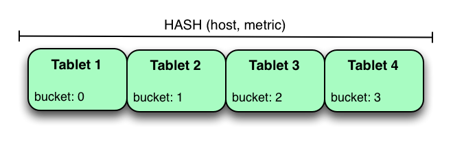
Hash Partitioning by `host` and `metric`

In the example above, the metrics table is hash partitioned on the host and metric columns into four buckets. Unlike the range partitioning example earlier, this partitioning strategy will spread writes over all tablets in the table evenly, which helps overall write throughput. Scans over a specific host and metric can take advantage of partition pruning by specifying equality predicates, reducing the number of scanned tablets to one. One issue to be careful of with a pure hash partitioning strategy, is that tablets could grow indefinitely as more and more data is inserted into the table. Eventually tablets will become too big for an individual tablet server to hold.

Although these examples number the tablets, in reality tablets are only given UUID identifiers. There is no natural ordering among the tablets in a hash partitioned table.

Hash and Range Partitioning Example

The previous examples showed how the metrics table could be range partitioned on the time column, or hash partitioned on the host and metric columns. These strategies have associated strength and weaknesses:

Table 2. Partitioning Strategies
Strategy	Writes	Reads	Tablet Growth
`range(time)`	✗ - all writes go to latest partition	✓ - time-bounded scans can be pruned	✓ - new tablets can be added for future time periods
`hash(host, metric)`	✓ - writes are spread evenly among tablets	✓ - scans on specific hosts and metrics can be pruned	✗ - tablets could grow too large

Hash partitioning is good at maximizing write throughput, while range partitioning avoids issues of unbounded tablet growth. Both strategies can take advantage of partition pruning to optimize scans in different scenarios. Using multilevel partitioning, it is possible to combine the two strategies in order to gain the benefits of both, while minimizing the drawbacks of each.

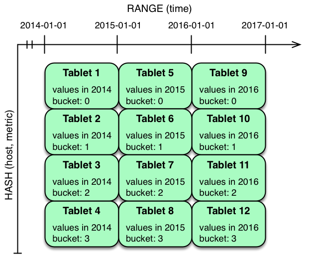
In the example above, range partitioning on the time column is combined with hash partitioning on the host and metric columns. This strategy can be thought of as having two dimensions of partitioning: one for the hash level and one for the range level. Writes into this table at the current time will be parallelized up to the number of hash buckets, in this case 4. Reads can take advantage of time bound and specific host and metric predicates to prune partitions. New range partitions can be added, which results in creating 4 additional tablets (as if a new column were added to the diagram).

Hash and Hash Partitioning Example

Kudu can support any number of hash partitioning levels in the same table, as long as the levels have no hashed columns in common.

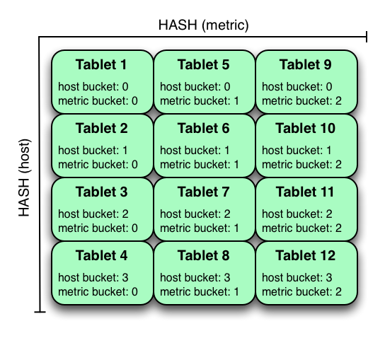
In the example above, the table is hash partitioned on host into 4 buckets, and hash partitioned on metric into 3 buckets, resulting in 12 tablets. Although writes will tend to be spread among all tablets when using this strategy, it is slightly more prone to hot-spotting than when hash partitioning over multiple independent columns, since all values for an individual host or metric will always belong to a single tablet. Scans can take advantage of equality predicates on the host and metric columns separately to prune partitions.

Multiple levels of hash partitioning can also be combined with range partitioning, which logically adds another dimension of partitioning.

Schema Alterations

You can alter a table’s schema in the following ways:

Rename the table
Rename primary key columns
Rename, add, or drop non-primary key columns
Add and drop range partitions

Multiple alteration steps can be combined in a single transactional operation.

Known Limitations

Kudu currently has some known limitations that may factor into schema design.

Number of Columns: By default, Kudu will not permit the creation of tables with more than 300 columns. We recommend schema designs that use fewer columns for best performance.
Size of Cells: No individual cell may be larger than 64KB before encoding or compression. The cells making up a composite key are limited to a total of 16KB after the internal composite-key encoding done by Kudu. Inserting rows not conforming to these limitations will result in errors being returned to the client.
Size of Rows: Although individual cells may be up to 64KB, and Kudu supports up to 300 columns, it is recommended that no single row be larger than a few hundred KB.
Valid Identifiers: Identifiers such as table and column names must be valid UTF-8 sequences and no longer than 256 bytes.
Immutable Primary Keys: Kudu does not allow you to update the primary key columns of a row.
Non-alterable Primary Key: Kudu does not allow you to alter the primary key columns after table creation.
Non-alterable Partitioning: Kudu does not allow you to change how a table is partitioned after creation, with the exception of adding or dropping range partitions.
Non-alterable Column Types: Kudu does not allow the type of a column to be altered.
Partition Splitting: Partitions cannot be split or merged after table creation.
Deleted row disk space is not reclaimed: The disk space occupied by a deleted row is only reclaimable via compaction, and only when the deletion’s age exceeds the "tablet history maximum age" (controlled by the --tablet_history_max_age_sec flag). Furthermore, Kudu currently only schedules compactions in order to improve read/write performance; a tablet will never be compacted purely to reclaim disk space. As such, range partitioning should be used when it is expected that large swaths of rows will be discarded. With range partitioning, individual partitions may be dropped to discard data and reclaim disk space. See KUDU-1625 for details.